Unsupervised Learning classify a given silhouette as one of three types of vehicle
Overview
The data contains features extracted from the silhouette of vehicles in different angles. The purpose is to classify a given silhouette as one of three types of vehicle, using a set of features extracted from the silhouette. The vehicle may be viewed from one of many different angles.
Solution
Import Necessary Libraries
 1# NumPy: For mathematical funcations, array, matrices operations
 2import numpy as np
 3
 4# Graph: Plotting graphs and other visula tools
 5import pandas as pd
 6import seaborn as sns
 7
 8# sns.set_palette("muted")
 9sns.set(color_codes=True)
10
11# color_palette = sns.color_palette()
12# To enable inline plotting graphs
13import matplotlib.pyplot as plt
14%matplotlib inline
General Util methods
1# Remove outliers from data frame
2def remove_outlier(df_in, col_name):
3    q1 = df_in[col_name].quantile(0.25)
4    q3 = df_in[col_name].quantile(0.75)
5    iqr = q3-q1 #Interquartile range
6    fence_low  = q1-1.5*iqr
7    fence_high = q3+1.5*iqr
8    df_out = df_in.loc[(df_in[col_name] > fence_low) & (df_in[col_name] < fence_high)]
9    return df_out
Load Data
 1# Load data set
 2# Import CSV data using pandas data frame
 3df_original = pd.read_csv('../vehicle-2.csv')
 4
 5# Print total columns
 6print("Total Colums in dataframe: ", len(df_original.columns))
 7
 8# Prepare columns names
 9df_original_columns = []
10for column in df_original.columns:
11    df_original_columns.append(column)
12
13
14
15print("Columns list {}".format(df_original_columns))
16print("***********************************************************************************************************************")
17
18# Prepare mapping of column names for quick access
19df_original_columns_map = {}
20map_index: int = 0
21for column in df_original_columns:
22    df_original_columns_map[map_index] = column
23    map_index = map_index + 1
24
25# print("Columns Map {}".format(df_original_columns_map))
26
27# We have separated out columns and its mapping from data, at any point of time during data analysis or cleaning we
28# can directly refer or get data from either index or column identifier
Total Colums in dataframe:  19
Columns list ['compactness', 'circularity', 'distance_circularity', 'radius_ratio', 'pr.axis_aspect_ratio', 'max.length_aspect_ratio', 'scatter_ratio', 'elongatedness', 'pr.axis_rectangularity', 'max.length_rectangularity', 'scaled_variance', 'scaled_variance.1', 'scaled_radius_of_gyration', 'scaled_radius_of_gyration.1', 'skewness_about', 'skewness_about.1', 'skewness_about.2', 'hollows_ratio', 'class']
***********************************************************************************************************************
Data pre-processing
Data shape
1df_original.shape
(846, 19)
Data Info
1df_original.info()
2# All columns are numeric in nature except target column
<class 'pandas.core.frame.DataFrame'>
RangeIndex: 846 entries, 0 to 845
Data columns (total 19 columns):
 #   Column                       Non-Null Count  Dtype
---  ------                       --------------  -----
 0   compactness                  846 non-null    int64
 1   circularity                  841 non-null    float64
 2   distance_circularity         842 non-null    float64
 3   radius_ratio                 840 non-null    float64
 4   pr.axis_aspect_ratio         844 non-null    float64
 5   max.length_aspect_ratio      846 non-null    int64
 6   scatter_ratio                845 non-null    float64
 7   elongatedness                845 non-null    float64
 8   pr.axis_rectangularity       843 non-null    float64
 9   max.length_rectangularity    846 non-null    int64
 10  scaled_variance              843 non-null    float64
 11  scaled_variance.1            844 non-null    float64
 12  scaled_radius_of_gyration    844 non-null    float64
 13  scaled_radius_of_gyration.1  842 non-null    float64
 14  skewness_about               840 non-null    float64
 15  skewness_about.1             845 non-null    float64
 16  skewness_about.2             845 non-null    float64
 17  hollows_ratio                846 non-null    int64
 18  class                        846 non-null    object
dtypes: float64(14), int64(4), object(1)
memory usage: 125.7+ KB
1df_original.head()
| compactness | circularity | distance_circularity | radius_ratio | pr.axis_aspect_ratio | max.length_aspect_ratio | scatter_ratio | elongatedness | pr.axis_rectangularity | max.length_rectangularity | scaled_variance | scaled_variance.1 | scaled_radius_of_gyration | scaled_radius_of_gyration.1 | skewness_about | skewness_about.1 | skewness_about.2 | hollows_ratio | class | |
|---|---|---|---|---|---|---|---|---|---|---|---|---|---|---|---|---|---|---|---|
| 0 | 95 | 48.0 | 83.0 | 178.0 | 72.0 | 10 | 162.0 | 42.0 | 20.0 | 159 | 176.0 | 379.0 | 184.0 | 70.0 | 6.0 | 16.0 | 187.0 | 197 | van |
| 1 | 91 | 41.0 | 84.0 | 141.0 | 57.0 | 9 | 149.0 | 45.0 | 19.0 | 143 | 170.0 | 330.0 | 158.0 | 72.0 | 9.0 | 14.0 | 189.0 | 199 | van |
| 2 | 104 | 50.0 | 106.0 | 209.0 | 66.0 | 10 | 207.0 | 32.0 | 23.0 | 158 | 223.0 | 635.0 | 220.0 | 73.0 | 14.0 | 9.0 | 188.0 | 196 | car |
| 3 | 93 | 41.0 | 82.0 | 159.0 | 63.0 | 9 | 144.0 | 46.0 | 19.0 | 143 | 160.0 | 309.0 | 127.0 | 63.0 | 6.0 | 10.0 | 199.0 | 207 | van |
| 4 | 85 | 44.0 | 70.0 | 205.0 | 103.0 | 52 | 149.0 | 45.0 | 19.0 | 144 | 241.0 | 325.0 | 188.0 | 127.0 | 9.0 | 11.0 | 180.0 | 183 | bus |
1# Data Describe
2df_original.describe().T
| count | mean | std | min | 25% | 50% | 75% | max | |
|---|---|---|---|---|---|---|---|---|
| compactness | 846.0 | 93.678487 | 8.234474 | 73.0 | 87.00 | 93.0 | 100.0 | 119.0 |
| circularity | 841.0 | 44.828775 | 6.152172 | 33.0 | 40.00 | 44.0 | 49.0 | 59.0 |
| distance_circularity | 842.0 | 82.110451 | 15.778292 | 40.0 | 70.00 | 80.0 | 98.0 | 112.0 |
| radius_ratio | 840.0 | 168.888095 | 33.520198 | 104.0 | 141.00 | 167.0 | 195.0 | 333.0 |
| pr.axis_aspect_ratio | 844.0 | 61.678910 | 7.891463 | 47.0 | 57.00 | 61.0 | 65.0 | 138.0 |
| max.length_aspect_ratio | 846.0 | 8.567376 | 4.601217 | 2.0 | 7.00 | 8.0 | 10.0 | 55.0 |
| scatter_ratio | 845.0 | 168.901775 | 33.214848 | 112.0 | 147.00 | 157.0 | 198.0 | 265.0 |
| elongatedness | 845.0 | 40.933728 | 7.816186 | 26.0 | 33.00 | 43.0 | 46.0 | 61.0 |
| pr.axis_rectangularity | 843.0 | 20.582444 | 2.592933 | 17.0 | 19.00 | 20.0 | 23.0 | 29.0 |
| max.length_rectangularity | 846.0 | 147.998818 | 14.515652 | 118.0 | 137.00 | 146.0 | 159.0 | 188.0 |
| scaled_variance | 843.0 | 188.631079 | 31.411004 | 130.0 | 167.00 | 179.0 | 217.0 | 320.0 |
| scaled_variance.1 | 844.0 | 439.494076 | 176.666903 | 184.0 | 318.00 | 363.5 | 587.0 | 1018.0 |
| scaled_radius_of_gyration | 844.0 | 174.709716 | 32.584808 | 109.0 | 149.00 | 173.5 | 198.0 | 268.0 |
| scaled_radius_of_gyration.1 | 842.0 | 72.447743 | 7.486190 | 59.0 | 67.00 | 71.5 | 75.0 | 135.0 |
| skewness_about | 840.0 | 6.364286 | 4.920649 | 0.0 | 2.00 | 6.0 | 9.0 | 22.0 |
| skewness_about.1 | 845.0 | 12.602367 | 8.936081 | 0.0 | 5.00 | 11.0 | 19.0 | 41.0 |
| skewness_about.2 | 845.0 | 188.919527 | 6.155809 | 176.0 | 184.00 | 188.0 | 193.0 | 206.0 |
| hollows_ratio | 846.0 | 195.632388 | 7.438797 | 181.0 | 190.25 | 197.0 | 201.0 | 211.0 |
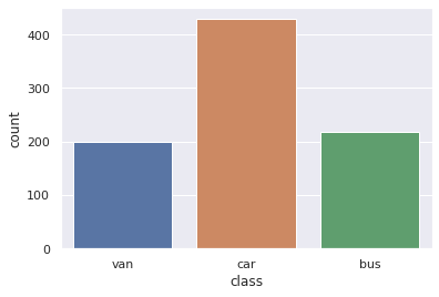
Target Colum Distribution
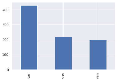
1pd.value_counts(df_original['class'])
car    429
bus    218
van    199
Name: class, dtype: int64
Count Plot For target column
1pd.value_counts(df_original["class"]).plot(kind="bar")
<matplotlib.axes._subplots.AxesSubplot at 0x7fc03fd39b50>
Checking for Missing value, duplicate data, incorrect data and perform data cleansing
Empty NA Values
1# Loading data in excel sheets quickly tells that there are Blank values in some columns
2# So print count of them as we are sure they exists
3
4df_original.isna().sum()
compactness                    0
circularity                    5
distance_circularity           4
radius_ratio                   6
pr.axis_aspect_ratio           2
max.length_aspect_ratio        0
scatter_ratio                  1
elongatedness                  1
pr.axis_rectangularity         3
max.length_rectangularity      0
scaled_variance                3
scaled_variance.1              2
scaled_radius_of_gyration      2
scaled_radius_of_gyration.1    4
skewness_about                 6
skewness_about.1               1
skewness_about.2               1
hollows_ratio                  0
class                          0
dtype: int64
Duplicates
1df_duplicates = df_original.duplicated()
2
3print('Number of duplicate rows = {}'.format(df_duplicates.sum()))
4
5# No duplicates
Number of duplicate rows = 0
Replace missing values with median
 1# Create a copy for df before operating on it
 2df_main = df_original.copy()
 3
 4# Replace all missing value from thei median
 5for column in df_original_columns:
 6    if df_main[column].isna().sum() > 0:
 7        median = df_main[column].median()
 8        df_main[column] = df_main[column].fillna(df_main[column].median())
 9
10
11
12# After replacement confirm that there are no mising values
13df_main.isna().sum()
compactness                    0
circularity                    0
distance_circularity           0
radius_ratio                   0
pr.axis_aspect_ratio           0
max.length_aspect_ratio        0
scatter_ratio                  0
elongatedness                  0
pr.axis_rectangularity         0
max.length_rectangularity      0
scaled_variance                0
scaled_variance.1              0
scaled_radius_of_gyration      0
scaled_radius_of_gyration.1    0
skewness_about                 0
skewness_about.1               0
skewness_about.2               0
hollows_ratio                  0
class                          0
dtype: int64
Lable encoding target column
1from sklearn import preprocessing
2target_column = 'class'
3le = preprocessing.LabelEncoder()
4le.fit(df_main[target_column])
5df_main[target_column] = le.transform(df_main[target_column])
6
7df_main.head()
| compactness | circularity | distance_circularity | radius_ratio | pr.axis_aspect_ratio | max.length_aspect_ratio | scatter_ratio | elongatedness | pr.axis_rectangularity | max.length_rectangularity | scaled_variance | scaled_variance.1 | scaled_radius_of_gyration | scaled_radius_of_gyration.1 | skewness_about | skewness_about.1 | skewness_about.2 | hollows_ratio | class | |
|---|---|---|---|---|---|---|---|---|---|---|---|---|---|---|---|---|---|---|---|
| 0 | 95 | 48.0 | 83.0 | 178.0 | 72.0 | 10 | 162.0 | 42.0 | 20.0 | 159 | 176.0 | 379.0 | 184.0 | 70.0 | 6.0 | 16.0 | 187.0 | 197 | 2 |
| 1 | 91 | 41.0 | 84.0 | 141.0 | 57.0 | 9 | 149.0 | 45.0 | 19.0 | 143 | 170.0 | 330.0 | 158.0 | 72.0 | 9.0 | 14.0 | 189.0 | 199 | 2 |
| 2 | 104 | 50.0 | 106.0 | 209.0 | 66.0 | 10 | 207.0 | 32.0 | 23.0 | 158 | 223.0 | 635.0 | 220.0 | 73.0 | 14.0 | 9.0 | 188.0 | 196 | 1 |
| 3 | 93 | 41.0 | 82.0 | 159.0 | 63.0 | 9 | 144.0 | 46.0 | 19.0 | 143 | 160.0 | 309.0 | 127.0 | 63.0 | 6.0 | 10.0 | 199.0 | 207 | 2 |
| 4 | 85 | 44.0 | 70.0 | 205.0 | 103.0 | 52 | 149.0 | 45.0 | 19.0 | 144 | 241.0 | 325.0 | 188.0 | 127.0 | 9.0 | 11.0 | 180.0 | 183 | 0 |
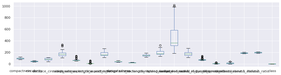
Presenceof outliers
1df_main.boxplot(figsize=(16,4))
<matplotlib.axes._subplots.AxesSubplot at 0x7fc03f2ae090>
Understanding the attributes
Pait Plot
1sns.pairplot(df_main,diag_kind='kde')
<seaborn.axisgrid.PairGrid at 0x7fc03ef2e2d0>
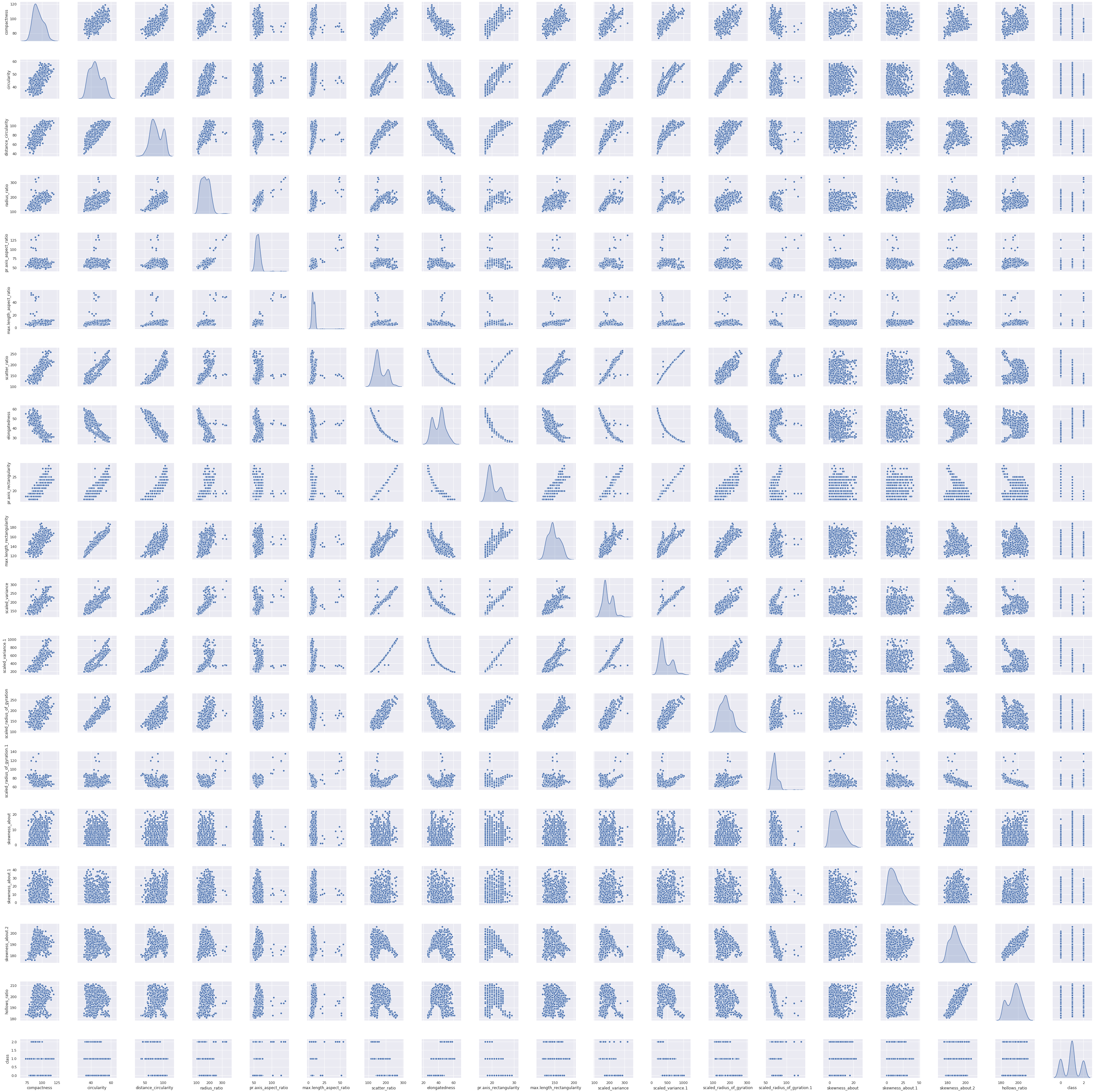
We can see there are some columns who has strong positive and negative correlations with them and some attributes where there is no relationship at all.
When there is not relation then distribution show values are saturated mostly in lower range
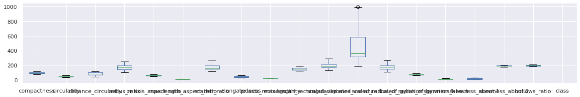
1
2# Treat outliers by removing them from data frame
3
4for name in df_original_columns:
5    df_main = remove_outlier(df_main, name)
6
7df_main.boxplot(figsize=(20,3))
<matplotlib.axes._subplots.AxesSubplot at 0x7fc034d37cd0>
Relationship Analysis between columns
1# Circularity
2pd.crosstab(df_original['class'], df_original['circularity'])
| circularity | 33.0 | 34.0 | 35.0 | 36.0 | 37.0 | 38.0 | 39.0 | 40.0 | 41.0 | 42.0 | ... | 50.0 | 51.0 | 52.0 | 53.0 | 54.0 | 55.0 | 56.0 | 57.0 | 58.0 | 59.0 |
|---|---|---|---|---|---|---|---|---|---|---|---|---|---|---|---|---|---|---|---|---|---|
| class | |||||||||||||||||||||
| bus | 0 | 0 | 1 | 3 | 7 | 6 | 5 | 6 | 11 | 22 | ... | 3 | 7 | 4 | 3 | 5 | 4 | 4 | 5 | 2 | 0 |
| car | 2 | 7 | 7 | 25 | 21 | 33 | 22 | 21 | 11 | 10 | ... | 12 | 22 | 24 | 27 | 34 | 29 | 11 | 7 | 3 | 1 |
| van | 0 | 2 | 8 | 13 | 14 | 8 | 15 | 15 | 13 | 15 | ... | 1 | 0 | 0 | 0 | 0 | 0 | 0 | 0 | 0 | 0 |
3 rows × 27 columns
1# elongatedness
2
3pd.crosstab(df_original['class'], df_original['elongatedness'])
| elongatedness | 26.0 | 27.0 | 28.0 | 29.0 | 30.0 | 31.0 | 32.0 | 33.0 | 34.0 | 35.0 | ... | 51.0 | 52.0 | 53.0 | 54.0 | 55.0 | 56.0 | 57.0 | 58.0 | 59.0 | 61.0 |
|---|---|---|---|---|---|---|---|---|---|---|---|---|---|---|---|---|---|---|---|---|---|
| class | |||||||||||||||||||||
| bus | 10 | 7 | 7 | 2 | 4 | 4 | 5 | 5 | 4 | 6 | ... | 0 | 0 | 0 | 0 | 0 | 0 | 0 | 0 | 0 | 0 |
| car | 0 | 0 | 0 | 0 | 46 | 69 | 39 | 23 | 17 | 19 | ... | 8 | 6 | 2 | 6 | 4 | 1 | 1 | 1 | 4 | 1 |
| van | 0 | 0 | 0 | 0 | 0 | 0 | 0 | 0 | 0 | 0 | ... | 10 | 14 | 8 | 4 | 6 | 5 | 11 | 3 | 0 | 0 |
3 rows × 35 columns
1sns.countplot(x='class',data=df_original)
<matplotlib.axes._subplots.AxesSubplot at 0x7fc030238c10>
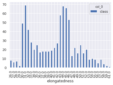
1my_tab = pd.crosstab(index = df_main["elongatedness"], columns="class")
2my_tab.plot.bar()
<matplotlib.axes._subplots.AxesSubplot at 0x7fc0301faa90>
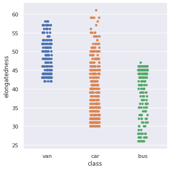
1sns.catplot(y='elongatedness', x='class', data=df_original)
<seaborn.axisgrid.FacetGrid at 0x7fc03015bbd0>
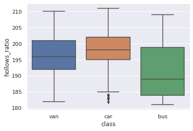
1sns.boxplot(y="hollows_ratio", x="class", data=df_original)
<matplotlib.axes._subplots.AxesSubplot at 0x7fc0300983d0>
Use PCA from scikit learn and elbow plot
Data standardization
1#Seperating independent and dependent variables
2
3df_main_x = df_main.copy().drop(['class'], axis = 1)
4
5
6df_main_y = df_main['class']
Applying standard scaler on independent variables
1from sklearn.preprocessing import StandardScaler
2
3sc = StandardScaler()
4
5main_x_std =  sc.fit_transform(df_main_x)
6
7cov_matrix = np.cov(main_x_std.T)
8
9print(cov_matrix)
Calculating Eigen Values & Vectors
1eigenvalues, eigenvectors = np.linalg.eig(cov_matrix)
 1# Step 3 (continued): Sort eigenvalues in descending order
 2
 3# Make a set of (eigenvalue, eigenvector) pairs
 4eig_pairs = [(eigenvalues[index], eigenvectors[:,index]) for index in range(len(eigenvalues))]
 5
 6# Sort the (eigenvalue, eigenvector) pairs from highest to lowest with respect to eigenvalue
 7eig_pairs.sort()
 8
 9eig_pairs.reverse()
10print(eig_pairs)
11
12# Extract the descending ordered eigenvalues and eigenvectors
13eigvalues_sorted = [eig_pairs[index][0] for index in range(len(eigenvalues))]
14eigvectors_sorted = [eig_pairs[index][1] for index in range(len(eigenvalues))]
15
16# Let's confirm our sorting worked, print out eigenvalues
17print('Eigenvalues in descending order: \n%s' %eigvalues_sorted)
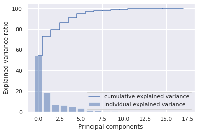
1total = sum(eigenvalues)
2var_exp = [( i /total ) * 100 for i in sorted(eigenvalues, reverse=True)]
3cum_var_exp = np.cumsum(var_exp)
4print("Cumulative Variance Explained", cum_var_exp)
Cumulative Variance Explained [ 54.1414912   72.83734035  79.57484836  85.9546281   90.96781645
  94.67377661  96.49487775  97.7654787   98.40655404  98.83353799
  99.18001751  99.4227584   99.58377841  99.72928046  99.83007959
  99.92588594  99.98250325 100.        ]
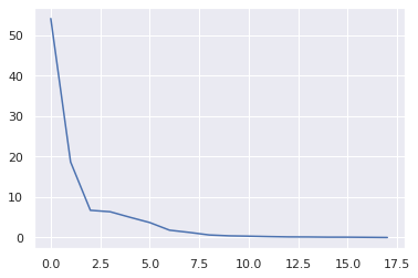
1plt.plot(var_exp)
[<matplotlib.lines.Line2D at 0x7fc02bfbb950>]
1plt.bar(range(0,18), var_exp, alpha=0.5, align='center', label='individual explained variance')
2plt.step(range(0,18),cum_var_exp, where= 'mid', label='cumulative explained variance')
3plt.ylabel('Explained variance ratio')
4plt.xlabel('Principal components')
5plt.legend(loc = 'best')
6plt.show()
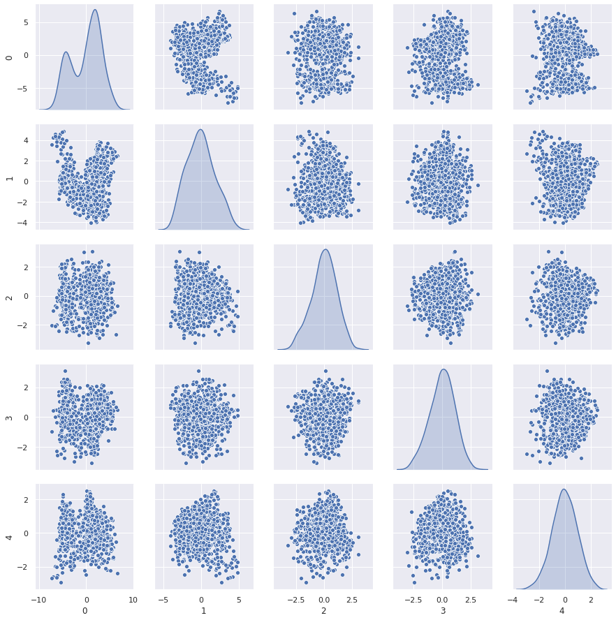
1# Reducing from 19 to 5 dimension space
2pca_reduced = np.array(eigvectors_sorted[0:5])
3# projecting original data into principal component dimensions
4main_x_4d = np.dot(main_x_std,pca_reduced.T)
5
6#converting array to dataframe for pairplot
7df_main_x_4d = pd.DataFrame(main_x_4d)
1sns.pairplot(df_main_x_4d,diag_kind='kde')
<seaborn.axisgrid.PairGrid at 0x7fc029f04a90>
 1from sklearn import model_selection
 2
 3test_size = 0.30 # taking 70:30 training and test set
 4seed = 7  # Random numbmer seeding for reapeatability of the code
 5X_train, X_test, y_train, y_test = model_selection.train_test_split(df_main_x, df_main_y, test_size=test_size, random_state=seed)
 6
 7# Let us build a linear regression model on the PCA dimensions
 8
 9# Import Linear Regression machine learning library
10from sklearn.linear_model import LinearRegression
11
12regression_model = LinearRegression()
13regression_model.fit(X_train, y_train)
14
15regression_model.coef_
16
17regression_model.score(X_test, y_test)
0.6336302682886086