1#Import Necessary Libraries
 2
 3# NumPy: For mathematical funcations, array, matrices operations
 4import numpy as np 
 5
 6# Graph: Plotting graphs and other visula tools
 7import pandas as pd
 8import seaborn as sns
 9
10# sns.set_palette("muted")
11# sns.set(color_codes=True)
12# sns.color_palette("colorblind", 10)
13
14
15# color_palette = sns.color_palette()
16# To enable inline plotting graphs
17import matplotlib.pyplot as plt
18%matplotlib inline
19
20
21# palette = sns.color_palette("muted")
22
23# sns.set_palette(palette)
24
25# sns.palplot(palette)
26
27flatui = ["#9b59b6", "#3498db", "#95a5a6", "#e74c3c", "#34495e", "#2ecc71"]
28
29sns.set_palette(flatui)
30
31sns.palplot(sns.color_palette())

 1# Custom terminal printer
 2
 3#Lets try to print unique values from object data type
 4from IPython.display import Markdown, display
 5
 6def printTextAsMarkdown(title, content, color=None):
 7    if title is None:
 8        colorStr = "<span style='color:{}'>{}</span>".format(color, content)
 9    else:    
10        colorStr = "**<span style='color:{}'>{}</span>** : {}".format(color, title, content)
11        
12    display(Markdown(colorStr))

 1# Load data set
 2# Import CSV data using pandas data frame
 3df_original = pd.read_csv('bank-full.csv')
 4
 5# Print total columns
 6print("Total Colums in dataframe: ", len(df_original.columns))
 7
 8# Prepare columns names
 9df_original_columns = []
10for column in df_original.columns:
11    df_original_columns.append(column)
12
13
14    
15print("Columns list {}".format(df_original_columns))
16print("***********************************************************************************************************************")
17
18# Prepare mapping of column names for quick access
19df_original_columns_map = {}
20map_index: int = 0
21for column in df_original_columns:
22    df_original_columns_map[map_index] = column
23    map_index = map_index + 1
24    
25print("Columns Map {}".format(df_original_columns_map))
26
27# We have separated out columns and its mapping from data, at any point of time during data analysis or cleaning we 
28# can directly refer or get data from either index or column identifier

1# Data frame general analysis
2df_original.head(16)

 1# Dataframe information
 2# Lets analyse data based on following conditions
 3# 1. Check whether all rows x colums are loaded as given in question, all data must match before we start to even operate on it.
 4# 2. Print shape of the data
 5# 8. Check data types of each field
 6# 3. Find presence of null or missing values.
 7# 4. Visually inspect data and check presense of Outliers if there are any and see are 
 8#    they enough to drop or need to consider during model building
 9# 5. Print shape of the data
10# 6. Do we need to consider all data columns given in data set for model building
11# 7. Find Corr, median, mean, std deviation, min, max for columns.
12
13df_original.info()

1# data types
2
3df_original.dtypes
4
5# also part of info indicating which are int nd object type though redundant.

1# Check presence of any null values
2
3df_original.isnull().values.any()
4
5# This return `False` it mean we do no have any present of null values

1# Check presence of missing value
2    
3df_original.isna().values.any()
4
5# This return `False` it mean we do no have any present of missing values

1# Shape of the data
2
3df_original.shape
4
5# we have 45211 rows and 17 columns

1# Check data loading and analyse data description
2
3df_original.describe()

1# Print Different data types from dataframe and its reference type
2
3df_original.dtypes.value_counts()

 1# Print unique for each column
 2
 3for name in df_original_columns:    
 4    if df_original[name].dtype == np.int64:
 5        #Sorting for better understanding
 6        sortedCategories =sorted(df_original[name].unique().tolist())
 7        
 8        formattedText = "has unique data in this range {}".format(sortedCategories)
 9        
10        printTextAsMarkdown(name, formattedText, color="red")
11        print("\n**************************************************************************************")

 1# We are most interested in qunie values of object data column, so lets filter out only object data type
 2# Priting ${df[name]} and its unique values
 3
 4# Container for object column type, later on while label encoding we need to convert only those column which are of type object
 5objectColumns = []
 6
 7for name in df_original_columns:    
 8    if df_original[name].dtype == np.object:
 9        
10        #Sorting for better understanding
11        sortedCategories =sorted(df_original[name].unique().tolist())
12        
13        formattedText = "has unique data in this range {}".format(sortedCategories)
14        
15        printTextAsMarkdown(name, formattedText, color="red")
16        
17        objectColumns.append(name)
18        print("\n**************************************************************************************")

1# Copy for original dataframe
2
3df_main = df_original.copy()

 1
 2
 3from sklearn import preprocessing
 4
 5# Create empty of of label encoders for different columns
 6# i wish to save each encoder corresponding to different colum title
 7
 8columnEncoders = {}
 9
10for name in objectColumns:
11    le = preprocessing.LabelEncoder()
12    # Fit encoder to pandas column
13    le.fit(df_main[name])
14    # apply transformation and assign it to df
15    df_main[name] = le.transform(df_main[name]) 
16    #put name and encoder in map 
17    columnEncoders[name] = le

1# Now lets revist basic operation on data frame
2
3df_main.head()
4
5# We can now see all data  into numeric form

1# Lets quickly print data types
2
3df_main.dtypes
4
5# Should print all int 

1# Let analyse more about data, 
2
3#df_main.describe() difficult to view hence lets apply transpose() to visually see it better
4
5df_main.describe().transpose()

1# Lets see response distribution for target column
2print(df_main['Target'].value_counts())
3
4sns.countplot(x='Target',data=df_original)
5
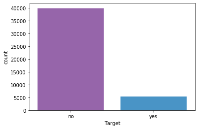
6# Here we have a kind of improper data, what ever model we build would 
7# be dominated by column have strong hold on `NO` on output variable becuase we see that data come from the range where
8# most of the people have not opted for Term Deposit

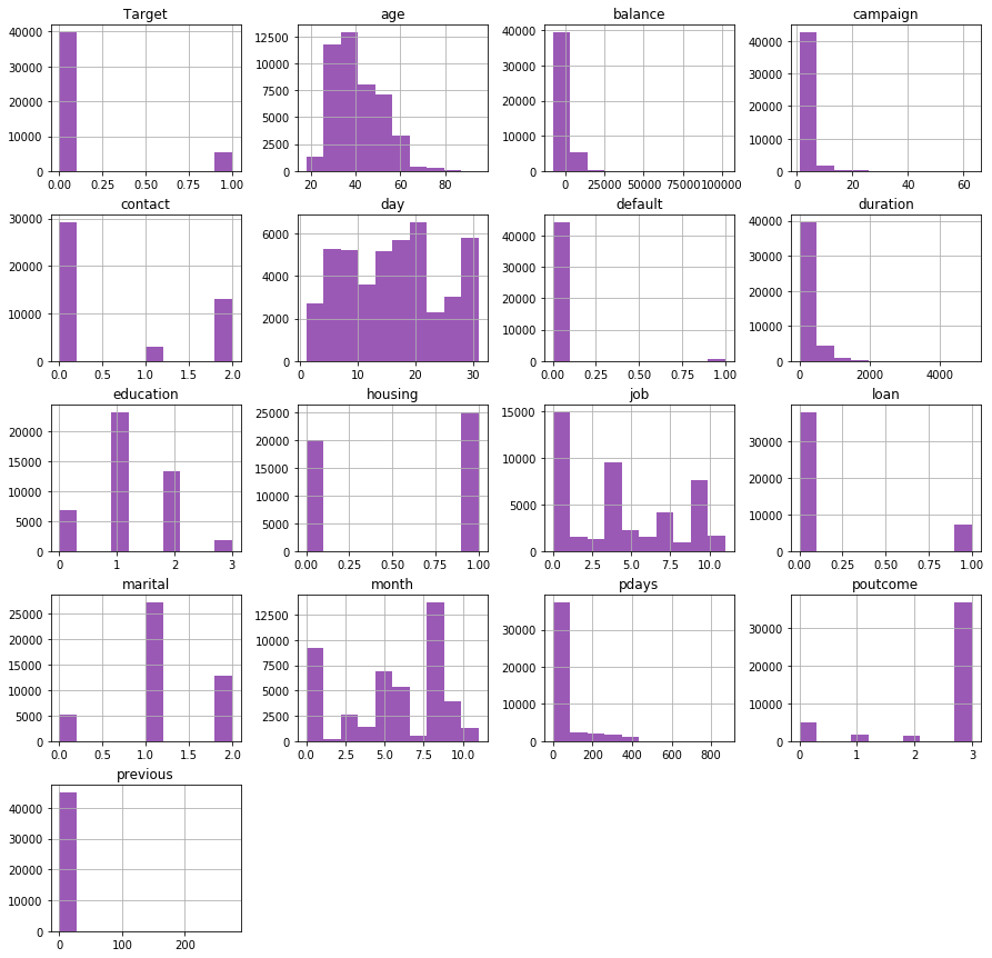
1# Histogram
2df_main.hist(figsize=(15,15))

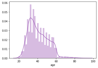
1sns.distplot(df_main['age'],kde=True)
2
3# We can conclude that data set has people raning from 20-60 and there are some outliers present as well
4# becuase the tail on right is spreading a little more

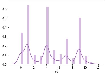
1sns.distplot(df_main['job'])
2# Looking at the graph we see that are multiple groups present in here, we have seen this and converted to categorical variable
3# lets print it from cached map `col`umnEncoders`
4print(columnEncoders['job'].classes_)

1# Relation between age, job to Term deposit
2sns.barplot('job','age',hue='Target',data=df_main,ci=None)
3print(columnEncoders['job'].classes_[4])
4
5# We can see that management people have opted for term deposit more

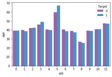
1# Finding relation between job and term deposit
2pd.crosstab(df_original['job'], df_original['Target'])
3
4# We here conclude that management, technician, blue-collar are some of the categories that tend to apply for term deposit.
5# This conclusion is based on that fact that their earning is on higher side. A general human assumption.

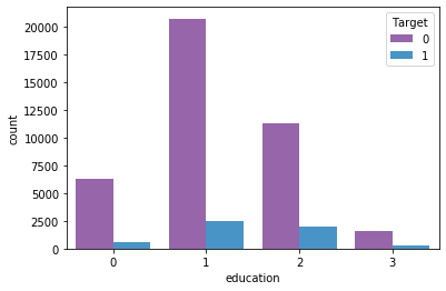
1# Lets analyse education-wise which category tend to apply more for term deposit respectively
2sns.countplot(x='education', hue='Target',data=df_main)
3print(columnEncoders['education'].classes_)
4
5# Here we conclude that the order of applyterm deposit secondary > tertiary > primary > unknown

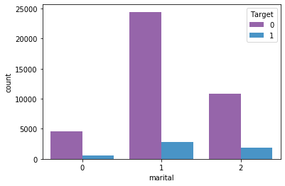
1# Lets analyse marital-status-wise which category tend to apply more for term deposit respectively
2
3sns.countplot(x='marital', hue='Target',data=df_main)#
4
5print(columnEncoders['marital'].classes_)
6
7# Here we conclude that the order of applyterm deposit is in married > single > divorced

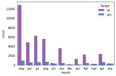
1pd.crosstab(df_original['Target'], df_original['month'])
2
3# We see here
4# - May has higher success and failure of Target values
5# - August has the second highest acceptanec value
6# But in terms of percentage acceptance august has higher value than may.

1# Deposit by months visual
2sns.countplot(x='month', hue='Target',data=df_original)

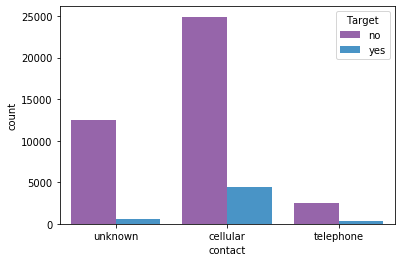
1# Checking if people who have given contants have got term deposit
2sns.countplot(x='contact', hue='Target',data=df_original)
3
4# This indicated who have registerd cellular contacts have slightly higer rate of applying for term deposit
5# This again tell us people who are working in higher job profile like management, technicians

1
2# Converting duration in dataset which is in seconds to minutes upto decimal ot 2 digits
3decimal_points = 2
4df_main['duration'] = df_main['duration'] / 60
5df_main['duration'] = df_main['duration'].apply(lambda x: round(x, decimal_points))
6
7df_main.head()

1# Balance colums seems to be dominating all other values lets scale it
2from sklearn.preprocessing import MinMaxScaler
3
4scaler = MinMaxScaler()
5
6df_main[['balance']] = scaler.fit_transform(df_main[['balance']])

1# Looking closely at our columns we see some columns prefixed with char `p`, reading from the problem
2# statement we came to know that these field are some kind of indicated of previous analysis or campaign 
3# like poutcome is not neccessarily should be part of train data model becuase this is not an attribute on input
4# but a conclusion on the previous analysis/campaign
5
6# So we can even build our data model removing these `p{x}` columns
7df_main.head()

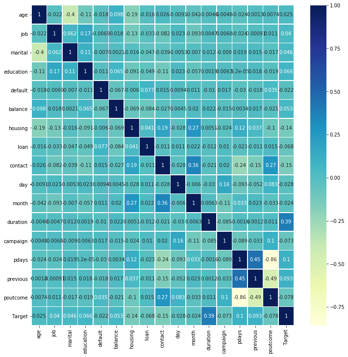
1df_main.corr()

1corr = df_main.corr()
2plt.figure(figsize = (12,12))
3
4sns.heatmap(corr, annot=True, linewidths=.5, cmap="YlGnBu")#, cbar=False)
5
6# Here we can simply reduce poutcome, pdays, previous, campaig

 1
 2# Training constants and general imports
 3
 4from sklearn.tree import DecisionTreeClassifier
 5from sklearn.ensemble import RandomForestClassifier
 6from sklearn.ensemble import AdaBoostClassifier
 7from sklearn.ensemble import BaggingClassifier
 8from sklearn.ensemble import GradientBoostingClassifier
 9
10
11
12from sklearn import metrics
13from sklearn.metrics import classification_report
14
15# taking 70:30 training and test set
16test_size = 0.30 
17
18# Random number seeding for reapeatability of the code
19seed = 2 # spirit and opportunity Mars exploration rovers
20
21
22def isqrt(n):
23    x = n
24    y = (x + 1) // 2
25    while y < x:
26        x = y
27        y = (x + n // x) // 2
28    return x

 1## Prepare input columns
 2df_main_x = df_main.copy()
 3
 4# Colums we are dropping which are mostly related to previous campaign
 5df_main_x = df_main_x.drop(['poutcome', 'duration', 'Target'], axis = 1) 
 6
 7# df_main_x_ary = np.asarray(df_main_x)
 8
 9df_main_y = df_original['Target']
10
11
12df_main_x.head()

1## Target column seperate
2df_main_y.head()

1
2from sklearn.model_selection import train_test_split
3
4X_train, X_test, y_train, y_test = \
5    train_test_split(np.asarray(df_main_x), np.asarray(df_main_y), test_size=test_size, random_state=seed)        

1# Holder class for data from different classifiers
2class EnsembleTechnique:
3    def __init__(self, score, prediction, accuracy, confusion_matrix, classification_report, n_estimators):
4        self.score = score
5        self.prediction = prediction
6        self.accuracy = accuracy
7        self.confusion_matrix = confusion_matrix
8        self.classification_report = classification_report
9        self.n_estimators = n_estimators

1rows = df_main_x.shape[0]
2print("Total rows {}".format(rows))
3maxLimit = isqrt(rows)
4print("Limit till we find Nestimators {}".format(maxLimit))
5
6# Result map to hold name and score for each model
7results = {}
8    

 1#Init
 2decisionTreeClassifier = DecisionTreeClassifier(criterion = 'entropy')
 3
 4#fit data
 5decisionTreeClassifier.fit(X_train, y_train)
 6
 7#Predict
 8dtc_y_pred = decisionTreeClassifier.predict(X_test)
 9
10# Model score
11dtc_model_score = decisionTreeClassifier.score(X_test , y_test)
12
13# Accuracy
14dtc_model_accuracy = metrics.accuracy_score(y_test, dtc_y_pred)
15
16
17print("Prediction: {}".format(dtc_y_pred))
18print("Score: {}".format(dtc_model_score))
19print("Accuracy {}".format(dtc_model_accuracy))
20print("Confusion metrix")
21print(metrics.confusion_matrix(y_test, dtc_y_pred))
22print(classification_report(y_test,dtc_y_pred))
23
24results['Decision Tree'] = dtc_model_score

 1
 2# determining n_estimators here, we should proceed with approach 2^n
 3# before stopping at the best outcome we should compare the result of previous outcome
 4previous = EnsembleTechnique(0.0, 0.0, 0.0, None, None, 0)
 5
 6counter = 1;
 7estimator = 0
 8while(estimator<maxLimit):
 9
10    estimator = pow(2, counter)
11    counter = counter + 1
12    
13    
14    #print("Estimating {}".format(estimator))
15    
16    #Init
17    randomForestClassifier = RandomForestClassifier(n_estimators=estimator)
18    #fit data
19    randomForestClassifier.fit(X_train, y_train)
20
21    #Predict
22    rfc_y_pred = randomForestClassifier.predict(X_test)
23
24    # Model score
25    rfc_model_score = randomForestClassifier.score(X_test , y_test)
26
27    # Accuracy
28    rfc_model_accuracy = metrics.accuracy_score(y_test, rfc_y_pred)
29    #print("Score {} for e {}".format(rfc_model_score, estimator))
30    #print(rfc_model_score)
31    if rfc_model_score > previous.score:
32        previous = EnsembleTechnique(rfc_model_score, rfc_y_pred, rfc_model_accuracy,
33                                    metrics.confusion_matrix(y_test, rfc_y_pred),
34                                    classification_report(y_test,rfc_y_pred), 
35                                    estimator)
36        
37    
38        
39    
40
41print("Prediction: {}".format(previous.prediction))
42print("Score: {}".format(previous.score))
43print("Accuracy {}".format(previous.accuracy))
44print("n estimators : {}".format(previous.n_estimators))
45print("Confusion metrix")
46print(previous.confusion_matrix)
47print(previous.classification_report)
48
49results['Random Forest'] = previous.score

 1
 2previous = EnsembleTechnique(0.0, 0.0, 0.0, None, None, 0)
 3
 4counter = 1;
 5estimator = 0
 6while(estimator<maxLimit):
 7
 8    estimator = pow(2, counter)
 9    counter = counter + 1
10    #Init
11    adaBoostClassifier = AdaBoostClassifier(n_estimators=estimator)
12    #fit data
13    adaBoostClassifier.fit(X_train, y_train)
14
15    #Predict
16    abc_y_pred = adaBoostClassifier.predict(X_test)
17
18    # Model score
19    abc_model_score = adaBoostClassifier.score(X_test , y_test)
20
21    # Accuracy
22    abc_model_accuracy = metrics.accuracy_score(y_test, abc_y_pred)
23    
24    if abc_model_score > previous.score:
25        previous = EnsembleTechnique(abc_model_score, abc_y_pred, abc_model_accuracy,
26                                    metrics.confusion_matrix(y_test, abc_y_pred),
27                                    classification_report(y_test, abc_y_pred), 
28                                    estimator)
29    
30    
31    
32    
33
34print("Prediction: {}".format(previous.prediction))
35print("Score: {}".format(previous.score))
36print("Accuracy {}".format(previous.accuracy))
37print("n estimators : {}".format(previous.n_estimators))
38print("Confusion metrix")
39print(previous.confusion_matrix)
40print(previous.classification_report)
41
42results['Adaboost Classifier'] = previous.score

 1
 2
 3previous = EnsembleTechnique(0.0, 0.0, 0.0, None, None, 0)
 4
 5counter = 1;
 6estimator = 0
 7while(estimator<maxLimit):
 8
 9    estimator = pow(2, counter)
10    counter = counter + 1
11    #Init
12    baggingClassifier = BaggingClassifier(n_estimators=estimator, max_samples= .7, bootstrap=True)
13    #fit data
14    baggingClassifier.fit(X_train, y_train)
15
16    #Predict
17    bc_y_pred = baggingClassifier.predict(X_test)
18
19    # Model score
20    bc_model_score = baggingClassifier.score(X_test , y_test)
21
22    # Accuracy
23    bc_model_accuracy = metrics.accuracy_score(y_test, bc_y_pred)
24    print("{} for n estimator {}".format(bc_model_score, estimator))
25    if bc_model_score > previous.score:
26        previous = EnsembleTechnique(bc_model_score, bc_y_pred, bc_model_accuracy,
27                                    metrics.confusion_matrix(y_test, bc_y_pred),
28                                    classification_report(y_test, bc_y_pred), 
29                                    estimator) 
30
31    
32        
33        
34results['Bagging Classifier'] = previous.score 
35print("Prediction: {}".format(previous.prediction))
36print("Score: {}".format(previous.score))
37print("Accuracy {}".format(previous.accuracy))
38print("n estimators : {}".format(previous.n_estimators))
39print("Confusion metrix")
40print(previous.confusion_matrix)
41print(previous.classification_report)

 1
 2previous = EnsembleTechnique(0.0, 0.0, 0.0, None, None, 0)
 3
 4counter = 1;
 5estimator = 0
 6while(estimator<maxLimit):
 7
 8    estimator = pow(2, counter)
 9    counter = counter + 1
10    #Init
11    gradientBoostClassifier = GradientBoostingClassifier(n_estimators=estimator, learning_rate = 0.05)
12    #fit data
13    gradientBoostClassifier.fit(X_train, y_train)
14
15    #Predict
16    gb_y_pred = gradientBoostClassifier.predict(X_test)
17
18    # Model score
19    gb_model_score = gradientBoostClassifier.score(X_test , y_test)
20
21    # Accuracy
22    gb_model_accuracy = metrics.accuracy_score(y_test, gb_y_pred)
23    
24    #print("{} for n estimator {}".format(bc_model_score, estimator))
25    if gb_model_score > previous.score:
26        previous = EnsembleTechnique(gb_model_score, gb_y_pred, gb_model_accuracy,
27                                    metrics.confusion_matrix(y_test,gb_y_pred),
28                                    classification_report(y_test, gb_y_pred), 
29                                    estimator) 
30
31
32results['Gradient Boost Classifier'] = previous.score 
33print("Prediction: {}".format(previous.prediction))
34print("Score: {}".format(previous.score))
35print("Accuracy {}".format(previous.accuracy))
36print("n estimators : {}".format(previous.n_estimators))
37print("Confusion metrix")
38print(previous.confusion_matrix)
39print(previous.classification_report)

1
2print("Model score are ")
3print(results)
4
5best_score = max(results, key=results.get);
6
7resultString = " has best score with accuracy **{}** ".format(results[best_score])
8
9printTextAsMarkdown(best_score, resultString, color="blue")